Listings, figures and delivery

A listing shows records, not statistics: every serious adverse event, every death, every protocol deviation. A reviewer reads it line by line. So every page needs the same layout: the same columns, the same widths, and the header again. A figure shows a pattern that a table hides: a trend over visits, or how fast events happen.

14.1 A listing by hand

A listing needs only a few PROC REPORT options, and always the same ones. They say which columns show a value only once, which column may wrap, and where a blank line goes. Learn them here; every company listing macro sets the same options for you.

/* Chapter 14: a listing of serious adverse events, by hand with PROC REPORT */

/* Step 010: the records to list, in the order to list them */
DATA sae;
  SET refadm.adae(WHERE=(saffl = "Y" AND aeser = "Y"));
  KEEP trtan trta usubjid aedecod astdt aendt aesev aeout;
RUN;
PROC SORT DATA=sae;
  BY trtan usubjid astdt aedecod;
RUN;

/* Step 020: print */
OPTIONS LS=132 PS=60 NOCENTER;
TITLE1 "Listing 16.2.7 Serious adverse events (safety population)";
PROC REPORT DATA=sae NOWD HEADLINE HEADSKIP SPLIT="|" SPACING=2;
  COLUMN trtan trta usubjid aedecod astdt aendt aesev aeout;
  DEFINE trtan   / ORDER NOPRINT;
  DEFINE trta    / ORDER   "Treatment"      WIDTH=20;
  DEFINE usubjid / ORDER   "Subject"        WIDTH=11;
  DEFINE aedecod / DISPLAY "Preferred term" WIDTH=30 FLOW;
  DEFINE astdt   / DISPLAY "Start"          WIDTH=9 FORMAT=DATE9.;
  DEFINE aendt   / DISPLAY "End"            WIDTH=9 FORMAT=DATE9.;
  DEFINE aesev   / DISPLAY "Severity"       WIDTH=8;
  DEFINE aeout   / DISPLAY "Outcome"        WIDTH=18 FLOW;
  BREAK AFTER usubjid / SKIP;
RUN;
TITLE;

What you should see:

Listing 16.2.7 Serious adverse events (safety population)

  Treatment             Subject      Preferred term                      Start        End  Severity  Outcome
  ---------------------------------------------------------------------------------------------------------------------

  Xanomeline Low Dose   01-718-1170  SYNCOPE                         12OCT2013  13OCT2013  SEVERE    RECOVERED/RESOLVED

  Xanomeline High Dose  01-709-1424  SYNCOPE                         07MAR2013  07MAR2013  MODERATE  RECOVERED/RESOLVED

                        01-718-1371  PARTIAL SEIZURES WITH           02JUN2013  05JUN2013  SEVERE    RECOVERED/RESOLVED
                                     SECONDARY GENERALISATION

The pilot study has three serious adverse events, and the listing shows all three. What each option does:

Step 010 sorts first. PROC REPORT prints the records in the order of the ORDER columns. Sort the data the same way, and the order is the one you chose, not an accident.
trtan as ORDER NOPRINT. The treatments print in the order of their numbers: placebo, low dose, high dose. That is not the alphabetical order of their names. The number itself does not print.
ORDER on trta and usubjid prints a value once per group: the high dose appears once for its two subjects.
FLOW with WIDTH=30 wraps a long preferred term inside its column, at a blank, instead of making the line wider than the page.
BREAK AFTER usubjid / SKIP writes a blank line after each subject, so a reviewer reads one subject at a time. HEADSKIP writes a blank line under the header.
LS=132 PS=60 set the page: 132 characters wide, 60 lines long. On every new page PROC REPORT prints the column headers again.

Exercise 14-1. List the subjects of the safety population who stopped the study because of an adverse event. In ADSL, that is dcreascd = "Adverse Event". Show their treatment and the date of their last dose (trtedt). How many subjects are there per treatment?

14.2 Figures with SGPLOT and LIFETEST

/* Chapter 14: two figures: mean weight change by visit, and a Kaplan-Meier plot */

/* graphs go to the WORK folder: every reader can write there */
ODS LISTING GPATH="%SYSFUNC(PATHNAME(WORK))";

/* Mean change from baseline in weight, by treatment and visit */
PROC MEANS DATA=refadm.advs(WHERE=(paramcd = "WEIGHT" AND anl01fl = "Y" AND 2 <= avisitn <= 26))
           NOPRINT NWAY;
  CLASS trtan trtp avisitn;
  VAR chg;
  OUTPUT OUT=chg_mean MEAN=mean STDERR=se N=n;
RUN;

DATA chg_plot;
  SET chg_mean;
  lo = mean - se;
  hi = mean + se;
RUN;

PROC PRINT DATA=chg_plot(WHERE=(avisitn = 24)) NOOBS;
  VAR trtp avisitn n mean se;
  FORMAT mean se 6.2;
RUN;

ODS GRAPHICS ON / WIDTH=16CM HEIGHT=10CM;
TITLE1 "Mean change from baseline in weight (kg), mean and standard error";
PROC SGPLOT DATA=chg_plot;
  SERIES  X=avisitn Y=mean / GROUP=trtp MARKERS;
  SCATTER X=avisitn Y=mean / GROUP=trtp YERRORLOWER=lo YERRORUPPER=hi;
  REFLINE 0 / AXIS=Y;
  XAXIS LABEL="Week" VALUES=(2 4 6 8 12 16 20 24 26);
  YAXIS LABEL="Change from baseline (kg)";
RUN;

/* Time to first dermatologic event: Kaplan-Meier estimate by treatment */
TITLE1 "Time to first dermatologic event";
ODS SELECT CensoredSummary Quartiles SurvivalPlot;
ODS OUTPUT Quartiles=km_q CensoredSummary=km_c;
PROC LIFETEST DATA=refadm.adtte PLOTS=SURVIVAL(ATRISK=0 to 210 by 30);
  TIME aval * cnsr(1);
  STRATA trtan;
RUN;
ODS SELECT ALL;
TITLE;

PROC PRINT DATA=km_q(WHERE=(percent = 50)) NOOBS; RUN;

What you should see: first a small table of the Week 24 means that the line plot draws,

TRTP	AVISITN	n	mean	se
Placebo	24	59	0.15	0.30
Xanomeline Low Dose	24	27	-0.34	0.39
Xanomeline High Dose	24	30	0.99	1.18

then the line plot:

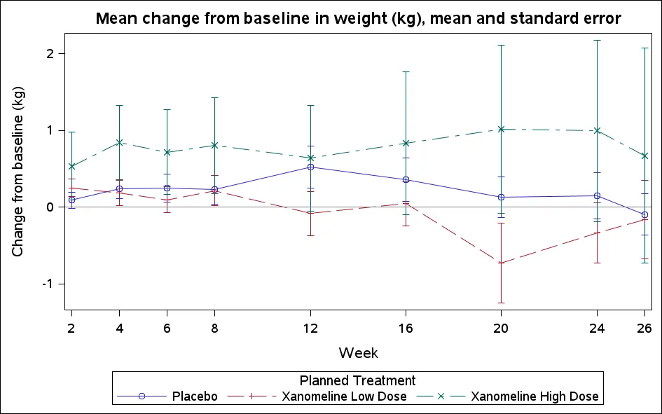
Line plot of mean change from baseline in weight with standard error bars, by planned treatment and week

The line plot as SAS draws it. Check the Week 24 points against the table above: 0.15 for placebo, -0.34 for the low dose, 0.99 for the high dose. The long bars of the active arms show how few subjects are left.

For the Kaplan-Meier analysis you see a summary of events and censored subjects per treatment,

Treatment	Total	Failed	Censored	Percent censored
Placebo (0)	86	29	57	66.28
Xanomeline Low Dose (54)	84	62	22	26.19
Xanomeline High Dose (81)	84	61	23	27.38
Total	254	152	102	40.16

the quartiles of the time to the first event, and the plot with the number of subjects at risk under it. The median time to the first dermatologic event:

Treatment	Median (days)	95% confidence interval
Placebo	not reached
Xanomeline Low Dose	33	27 to 48
Xanomeline High Dose	36	23 to 46

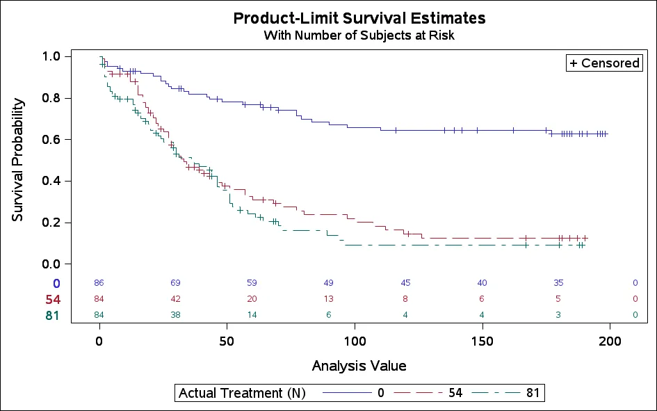
Kaplan-Meier plot of the time to the first dermatologic event by treatment, with the number of subjects at risk

The Kaplan-Meier plot from PROC LIFETEST. Under it is the number of subjects at risk: 86, 84 and 84 at day 0, and 49 on placebo at day 90. SAS labels the treatments with their codes (0, 54, 81) and the time axis “Analysis Value”. In a report, attach a format to TRTAN and label AVAL “Days”.

On placebo, only 29 of 86 subjects had the event. That is fewer than half, so the curve never falls to 50%. The median is not reached. SAS prints a missing value; the table of the report must say “not reached”, not ”.”.

Three habits for figures:

Compute first, then draw. PROC MEANS writes the means and standard errors to a data set, and SGPLOT only draws it. You can print and check every point of the plot before you look at the picture.
Write the images where you may write. The first line sends the image files to the WORK folder. Without it, a server session writes into the folder SAS started in, and on SAS OnDemand that fails with ERROR: Cannot write image to ....
Look at the n. At Week 24 the low dose has 27 subjects with a weight, and placebo has 59. Many subjects of the active arms stopped early. A mean of few, selected subjects needs that warning next to it.

Exercise 14-2. Change the line plot to show systolic blood pressure, one line per treatment, with the standard error as bars.

Exercise 14-3. In the Kaplan-Meier plot, how many placebo subjects are still at risk at day 90? Read it from the at-risk table under the plot, then check it with a DATA step or PROC SQL on ADTTE.

14.3 Delivery: the table as an RTF file

The statistician and the medical writer do not read the SAS output window. They get a file: in most companies RTF, which opens in Word, sometimes PDF. Each table, listing and figure is one file, with the study name, the page number and the program name on every page. SAS writes these files with ODS, the Output Delivery System. ODS RTF opens a file, every procedure after it writes into the file, and ODS RTF CLOSE finishes it. Here is the demographics table of section 13.5 as RTF and PDF:

/* Chapter 14: the demographics table as an RTF file and a PDF file (needs DM_ROWS and DM_BIGN from 13_4) */

/* Step 010: one column per treatment, as in step 010 of %m_report */
PROC SORT DATA=dm_rows OUT=rtf_010; BY ord sub label; RUN;
PROC TRANSPOSE DATA=rtf_010 OUT=rtf_dm(DROP=_name_) PREFIX=c;
  BY ord sub label;
  ID col;
  VAR value;
RUN;

/* Step 020: the big N of each column as a macro variable: n0, n54, n81 */
DATA _NULL_;
  SET dm_bign;
  CALL SYMPUTX(CATS("n", col), bign);
RUN;

/* Step 030: the output files. The FILENAME tells the log where they are */
/* The output folder: the folder of the program if SAS may write there (DataStep Studio runs */
/* a program in its own folder and brings the files back), else your SAS home folder.        */
DATA _NULL_;
  LENGTH outdir $256;
  rc  = FILENAME("_probe", "_probe.txt");
  fid = FOPEN("_probe", "o");
  IF fid > 0 THEN DO;
    outdir = ".";
    rc = FCLOSE(fid);
    rc = FDELETE("_probe");
  END;
  ELSE outdir = SYSGET("HOME");
  rc = FILENAME("_probe");
  CALL SYMPUTX("outdir", outdir);
RUN;
FILENAME rtfout "&outdir./t_14_1_1_demog.rtf";
FILENAME pdfout "&outdir./t_14_1_1_demog.pdf";
%PUT NOTE: RTF file: %SYSFUNC(PATHNAME(rtfout));

/* Step 040: titles, footnotes and page x of y. ^ starts an ODS escape */
/* landscape with 1 inch margins: 11 - 2 = 9 inches for the table */
OPTIONS NODATE NONUMBER ORIENTATION=LANDSCAPE LEFTMARGIN=1IN RIGHTMARGIN=1IN TOPMARGIN=1IN BOTTOMMARGIN=1IN;
ODS ESCAPECHAR="^";
TITLE1    J=L "CDISCPILOT01" J=R "Page ^{thispage} of ^{lastpage}";
TITLE2    J=C "Table 14.1.1 Demographics";
TITLE3    J=C "Safety population";
FOOTNOTE1 J=L "N = subjects in the safety population. n (%) = subjects in the category, percent of N.";
FOOTNOTE2 J=L "Program: 14_3_rtf_demog.sas";

/* Step 050: one PROC REPORT, two files */
ODS LISTING CLOSE;
ODS RTF FILE=rtfout STYLE=Journal;
ODS PDF FILE=pdfout STYLE=Journal;
PROC REPORT DATA=rtf_dm NOWD SPLIT="|" MISSING
            STYLE(report)=[font_face="Courier New" font_size=9pt]
            STYLE(header)=[font_face="Courier New" font_size=9pt just=c]
            STYLE(column)=[font_face="Courier New" font_size=9pt];
  COLUMN ord sub label ("Treatment" c0 c54 c81);
  DEFINE ord   / ORDER NOPRINT;
  DEFINE sub   / ORDER NOPRINT;
  DEFINE label / DISPLAY " " STYLE(column)=[cellwidth=3.2in asis=on just=l];
  DEFINE c0    / DISPLAY "Placebo|(N=&n0.)"              STYLE(column)=[cellwidth=1.75in just=c];
  DEFINE c54   / DISPLAY "Xanomeline Low Dose|(N=&n54.)"  STYLE(column)=[cellwidth=1.75in just=c];
  DEFINE c81   / DISPLAY "Xanomeline High Dose|(N=&n81.)" STYLE(column)=[cellwidth=1.75in just=c];
  /* the widths add up to 3.2 + 3 x 1.75 = 8.45 inches: less than the 9 inches of the page */
  /* the heading line of each section in bold */
  COMPUTE label;
    IF sub = 0 THEN CALL DEFINE(_COL_, "style", "style=[font_weight=bold]");
  ENDCOMP;
  /* an empty line after each section */
  COMPUTE AFTER ord;
    LINE " ";
  ENDCOMP;
RUN;
ODS PDF CLOSE;
ODS RTF CLOSE;
ODS LISTING;
TITLE;
FOOTNOTE;

What you should see: in the log, the place of the file, for example NOTE: RTF file: .../t_14_1_1_demog.rtf. DataStep Studio runs a program in its own folder on the server. The files land next to the program and come back to your computer (chapter 20). In SAS Studio or a batch run, SAS may not write in that folder. Then the program writes to your SAS home folder, and the log shows that path.

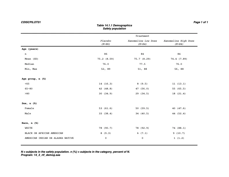
Page 1 of t_14_1_1_demog.pdf, made by this program on SAS OnDemand. It shows “Page 1 of 1”, the header “Treatment” above the three columns, the big N in each header, and the section headings in bold. The numbers are those of section 13.5.

Step by step:

The DATA _NULL_ step before the FILENAMEs tests if SAS may write in the program’s folder. FOPEN opens a test file for output. If that works, outdir is ., the program’s folder. If not, outdir is your home folder, from SYSGET("HOME"). FDELETE removes the test file.
FILENAME gives the file a short name, rtfout. PATHNAME(rtfout) returns the full path, for the log.
OPTIONS NODATE NONUMBER ORIENTATION=LANDSCAPE and the four margins. The title line shows no date and no SAS page number, because the title has its own. The pages are landscape, with 1 inch of margin on each side.
ODS ESCAPECHAR="^" makes ^ a special character in text. ^{thispage} and ^{lastpage} are the page number and the number of pages: Word fills them in when it shows the file. That is the “Page 1 of 3” line of every table.
TITLE1 J=L "..." J=R "...": J=L puts the text at the left, J=R at the right of the same line. FOOTNOTE works the same way at the bottom of the page.
ODS LISTING CLOSE stops the normal output while the file is open; ODS LISTING at the end starts it again. Two destinations can be open at the same time: one PROC REPORT writes the RTF file and the PDF file.
STYLE=Journal is a plain style with lines above and below the header, close to what most companies use. Your company has its own style.

The PROC REPORT step is the one of %m_report, with four additions for a document:

STYLE(report)=[...], STYLE(header)=[...], STYLE(column)=[...] set the font of the whole table, of the headers and of the cells. In an RTF file WIDTH= means nothing: cellwidth=1.75in sets the width of a column.
The widths must fit the page. Landscape paper is 11 inches wide; LEFTMARGIN=1IN RIGHTMARGIN=1IN leave 9 inches. Here the columns take 3.2 + 3 × 1.75 = 8.45 inches. The first version of this program used percent widths that added up to 100 %. With the space around each cell, the table was wider than the page. SAS then puts the columns that do not fit on the next page, and page 1 shows only the labels. Add up your widths.
asis=on keeps the leading blanks of the label: without it, ” Mean (SD)” would lose its indent.
("Treatment" c0 c54 c81) in the COLUMN statement puts one header, “Treatment”, above the three treatment columns.
COMPUTE label ... CALL DEFINE(_COL_, "style", ...) changes one cell while PROC REPORT writes it: the heading line of each section (sub = 0) is bold. A COMPUTE block is a small DATA step that runs for each row of the report.

Exercise 14-4. Copy 14_3_rtf_demog.sas and change the style from Journal to RTF. What changes in the PDF file?

14.4 PROC REPORT in depth: the listing as an RTF file

A listing has many pages. Three more parts of PROC REPORT handle them: a page variable, a BREAK with / PAGE, and COMPUTE AFTER for a line at the end.

/* Chapter 14: the listing of serious adverse events as an RTF file and a PDF file (needs SAE from 14_1) */

/* Step 010: a page variable, a new page for each treatment, and a counter for the total line */
DATA rtf_sae;
  SET sae;
  BY trtan;
  RETAIN pg 0;
  IF FIRST.trtan THEN pg + 1;
  one = 1;
RUN;

/* Step 020: the output files */
/* The output folder: the folder of the program if SAS may write there (DataStep Studio runs */
/* a program in its own folder and brings the files back), else your SAS home folder.        */
DATA _NULL_;
  LENGTH outdir $256;
  rc  = FILENAME("_probe", "_probe.txt");
  fid = FOPEN("_probe", "o");
  IF fid > 0 THEN DO;
    outdir = ".";
    rc = FCLOSE(fid);
    rc = FDELETE("_probe");
  END;
  ELSE outdir = SYSGET("HOME");
  rc = FILENAME("_probe");
  CALL SYMPUTX("outdir", outdir);
RUN;
FILENAME rtfout "&outdir./l_16_2_7_sae.rtf";
FILENAME pdfout "&outdir./l_16_2_7_sae.pdf";
%PUT NOTE: RTF file: %SYSFUNC(PATHNAME(rtfout));

/* Step 030: titles and footnotes, page x of y */
/* landscape with 1 inch margins: 9 inches for the listing */
OPTIONS NODATE NONUMBER ORIENTATION=LANDSCAPE LEFTMARGIN=1IN RIGHTMARGIN=1IN TOPMARGIN=1IN BOTTOMMARGIN=1IN;
ODS ESCAPECHAR="^";
TITLE1    J=L "CDISCPILOT01" J=R "Page ^{thispage} of ^{lastpage}";
TITLE2    J=C "Listing 16.2.7 Serious adverse events";
TITLE3    J=C "Safety population";
FOOTNOTE1 J=L "Start and end are the analysis dates ASTDT and AENDT. An empty end date: the event had not ended.";
FOOTNOTE2 J=L "Program: 14_4_rtf_listing.sas";

/* Step 040: the report */
ODS LISTING CLOSE;
ODS RTF FILE=rtfout STYLE=Journal;
ODS PDF FILE=pdfout STYLE=Journal;
PROC REPORT DATA=rtf_sae NOWD SPLIT="|" MISSING
            STYLE(report)=[font_face="Courier New" font_size=9pt]
            STYLE(header)=[font_face="Courier New" font_size=9pt just=l]
            STYLE(column)=[font_face="Courier New" font_size=9pt];
  COLUMN pg trtan trta usubjid aedecod astdt aendt aesev aeout one;
  DEFINE pg      / ORDER NOPRINT;
  DEFINE trtan   / ORDER NOPRINT;
  DEFINE trta    / ORDER   "Treatment"      STYLE(column)=[cellwidth=1.6in];
  DEFINE usubjid / ORDER   "Subject"        STYLE(column)=[cellwidth=1.0in];
  DEFINE aedecod / DISPLAY "Preferred term" STYLE(column)=[cellwidth=2.0in];
  DEFINE astdt   / DISPLAY "Start"          FORMAT=DATE9. STYLE(column)=[cellwidth=0.85in];
  DEFINE aendt   / DISPLAY "End"            FORMAT=DATE9. STYLE(column)=[cellwidth=0.85in];
  DEFINE aesev   / DISPLAY "Severity"       STYLE(column)=[cellwidth=0.75in];
  DEFINE aeout   / DISPLAY "Outcome"        STYLE(column)=[cellwidth=1.5in];
  DEFINE one     / ANALYSIS SUM NOPRINT;
  /* the widths add up to 8.55 inches: less than the 9 inches of the page */
  /* a new page for each value of pg */
  BREAK AFTER pg / PAGE;
  /* an empty line after each subject */
  COMPUTE AFTER usubjid;
    LINE " ";
  ENDCOMP;
  /* one line at the end of the report: the number of events listed */
  COMPUTE AFTER;
    LINE "Number of serious adverse events listed: " one.sum 3.;
  ENDCOMP;
RUN;
ODS PDF CLOSE;
ODS RTF CLOSE;
ODS LISTING;
TITLE;
FOOTNOTE;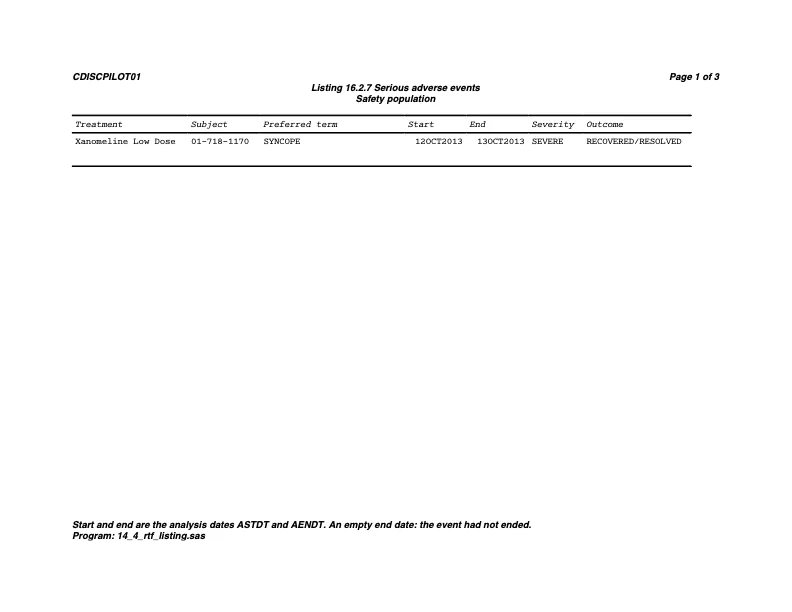

Page 1 of l_16_2_7_sae.pdf: “Page 1 of 3”, because each of the three treatments starts a new page. All seven columns fit in the 9 inches.

Every DEFINE has a usage. The four you need:

Usage	What PROC REPORT does with the variable	In this listing
`ORDER`	sorts the rows by it, prints a value only when it changes	`trta`, `usubjid`
`DISPLAY`	prints the value on every row	`aedecod`, `astdt`
`ANALYSIS`	a number to add up (`SUM`, `MEAN`) for break lines	`one`
`GROUP`	one row per value, with the `ANALYSIS` variables summed	(not used here: for a summary table)

NOPRINT keeps a variable in the report without a column: pg and trtan decide the order and the pages, but nobody needs to see them.

BREAK AFTER pg / PAGE starts a new page when pg changes. Step 010 adds 1 to pg at the first record of each treatment, so each treatment starts on a new page. To break by a number of subjects instead, count subjects and set pg = CEIL(count / 10).
COMPUTE AFTER usubjid; LINE " "; ENDCOMP; writes an empty line after each subject. In the output window BREAK ... / SKIP did that; RTF ignores SKIP, so use LINE.
COMPUTE AFTER; ... ENDCOMP; without a variable runs once, at the end of the report. one.sum is the sum of one: the number of rows listed. A listing that says how many records it has is easy to check against the data.

Exercise 14-5. List the severe treatment emergent adverse events (aesev = "SEVERE" in ADAE) the same way, with a new page for every 10 subjects. How many records, subjects and pages?

14.5 A figure in the document

ODS RTF takes figures too. ODS GRAPHICS ON / WIDTH= HEIGHT= sets the size of the picture. Two options decide where the titles go:

NOGTITLE NOGFOOTNOTE: without them, SAS draws the titles inside the picture. Then ^{thispage} is only text in an image, and the first version of this program printed “Page of” with no numbers. With them, the titles stay text on the page.
BODYTITLE (RTF only): the titles go into the page above the graph, not into the Word page header.

/* Chapter 14: the weight figure as an RTF file and a PDF file (needs CHG_PLOT from 14_2) */

/* The output folder: the folder of the program if SAS may write there (DataStep Studio runs */
/* a program in its own folder and brings the files back), else your SAS home folder.        */
DATA _NULL_;
  LENGTH outdir $256;
  rc  = FILENAME("_probe", "_probe.txt");
  fid = FOPEN("_probe", "o");
  IF fid > 0 THEN DO;
    outdir = ".";
    rc = FCLOSE(fid);
    rc = FDELETE("_probe");
  END;
  ELSE outdir = SYSGET("HOME");
  rc = FILENAME("_probe");
  CALL SYMPUTX("outdir", outdir);
RUN;
FILENAME rtfout "&outdir./f_14_2_1_weight.rtf";
FILENAME pdfout "&outdir./f_14_2_1_weight.pdf";
%PUT NOTE: RTF file: %SYSFUNC(PATHNAME(rtfout));

OPTIONS NODATE NONUMBER ORIENTATION=LANDSCAPE LEFTMARGIN=1IN RIGHTMARGIN=1IN TOPMARGIN=1IN BOTTOMMARGIN=1IN;
ODS ESCAPECHAR="^";
TITLE1    J=L "CDISCPILOT01" J=R "Page ^{thispage} of ^{lastpage}";
TITLE2    J=C "Figure 14.2.1 Mean change from baseline in weight (kg)";
TITLE3    J=C "Safety population, mean and standard error";
FOOTNOTE1 J=L "Program: 14_5_rtf_figure.sas";

/* NOGTITLE NOGFOOTNOTE: the titles stay text on the page, not part of the picture, so Page x of y works. */
/* BODYTITLE: in RTF the titles go into the page above the graph, not into the page header.             */
ODS LISTING CLOSE;
ODS GRAPHICS ON / WIDTH=22CM HEIGHT=11CM;
ODS RTF FILE=rtfout STYLE=Journal BODYTITLE NOGTITLE NOGFOOTNOTE;
ODS PDF FILE=pdfout STYLE=Journal NOGTITLE NOGFOOTNOTE;
PROC SGPLOT DATA=chg_plot NOAUTOLEGEND;
  SERIES  X=avisitn Y=mean / GROUP=trtp MARKERS NAME="lines";
  SCATTER X=avisitn Y=mean / GROUP=trtp YERRORLOWER=lo YERRORUPPER=hi;
  REFLINE 0 / AXIS=Y;
  XAXIS LABEL="Week" VALUES=(2 4 6 8 12 16 20 24 26);
  YAXIS LABEL="Change from baseline (kg)";
  KEYLEGEND "lines" / TITLE="";
RUN;
ODS PDF CLOSE;
ODS RTF CLOSE;
ODS LISTING;
TITLE;
FOOTNOTE;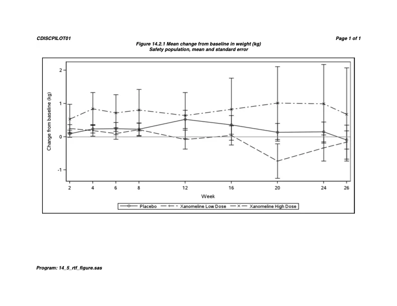

Page 1 of f_14_2_1_weight.pdf: the titles and the page number above the graph, the program name at the bottom.

Before you send a file, open it. Check four things. The page numbers count to the right total. No column is cut. The big N in the header matches the table. The title has the number and the population of the shell.

Exercise 14-6. Put the TEAE table of 13_2_table_ae.sas into an RTF file with “Page x of y” in the title. How many pages does it have?

Exercises

Each exercise is next to the program it changes. 14-1 uses 14_1_listing.sas. 14-2 and 14-3 use 14_2_figures.sas. 14-4 to 14-6 use the RTF programs 14_3 to 14_5. The answers are in Answers, Part III.