Tables by hand, then with study macros

Every company has a TLF macro library, and every library is different. What they do is the same everywhere. This chapter shows that by hand. First come two tables without any macro. Then you write four small study macros, because the same code came back. When you can do it by hand, you can read any library, and you can do what the library cannot.

13.1 The four jobs of a table program

A summary table looks simple: rows of statistics, one column per treatment. Behind it are four jobs, always in this order:

Population and big N. Which subjects, and how many in each column. The header says Placebo (N=86), and every percent divides by that 86.
Compute the statistics: n, mean, median for numbers; counts and percents for categories.
Arrange them in a layout data set: one row per printed line, one column per treatment, every number already formatted as text.
Print the layout data set with PROC REPORT.

Keep the jobs apart. When a reviewer questions a number, look at job 2. When the shell (the mock table from the statistician) changes the order of the rows, change job 3. When the page changes, change job 4, and no number moves.

13.2 A demographics table by hand

/* Chapter 13: a demographics table in plain SAS: statistics, a layout data set, PROC REPORT */

/* Step 010: big N per treatment into macro variables */
PROC SQL NOPRINT;
  SELECT COUNT(DISTINCT usubjid) INTO :n0 TRIMMED FROM refadm.adsl WHERE saffl = "Y" AND trt01an = 0;
  SELECT COUNT(DISTINCT usubjid) INTO :n54 TRIMMED FROM refadm.adsl WHERE saffl = "Y" AND trt01an = 54;
  SELECT COUNT(DISTINCT usubjid) INTO :n81 TRIMMED FROM refadm.adsl WHERE saffl = "Y" AND trt01an = 81;
QUIT;

/* Step 020: age, a continuous variable: n, mean (SD), median, min and max */
PROC MEANS DATA=refadm.adsl(WHERE=(saffl = "Y")) NOPRINT NWAY;
  CLASS trt01an;
  VAR age;
  OUTPUT OUT=age_stat N=n MEAN=mean STD=sd MEDIAN=median MIN=min MAX=max;
RUN;

DATA age_rows;
  LENGTH label $40 value $20;
  SET age_stat;
  ord = 1;
  label = "  n";              value = PUT(n, 3.);                                      sub = 1; OUTPUT;
  label = "  Mean (SD)";      value = CATX(" ", PUT(mean, 5.1), CATS("(", PUT(sd, 5.2), ")")); sub = 2; OUTPUT;
  label = "  Median";         value = PUT(median, 5.1);                                sub = 3; OUTPUT;
  label = "  Min, Max";       value = CATX(", ", PUT(min, 3.), PUT(max, 3.));          sub = 4; OUTPUT;
  KEEP trt01an ord sub label value;
RUN;

/* Step 030: sex, a categorical variable: n (%) of the big N */
PROC FREQ DATA=refadm.adsl(WHERE=(saffl = "Y")) NOPRINT;
  TABLES trt01an * sex / OUT=sex_cnt;
RUN;

DATA sex_rows;
  LENGTH label $40 value $20;
  SET sex_cnt;
  ord = 2;
  IF      trt01an = 0  THEN bign = &n0.;
  ELSE IF trt01an = 54 THEN bign = &n54.;
  ELSE IF trt01an = 81 THEN bign = &n81.;
  IF sex = "F" THEN DO; label = "  Female"; sub = 1; END;
  ELSE              DO; label = "  Male";   sub = 2; END;
  value = CATX(" ", PUT(count, 3.), CATS("(", PUT(count / bign * 100, 5.1), ")"));
  KEEP trt01an ord sub label value;
RUN;

/* Step 040: the layout data set: one row per table line, one column per treatment */
DATA heads;
  LENGTH label $40;
  ord = 1; sub = 0; label = "Age (years)"; OUTPUT;
  ord = 2; sub = 0; label = "Sex, n (%)";  OUTPUT;
RUN;

DATA long;
  SET age_rows sex_rows;
RUN;
PROC SORT DATA=long; BY ord sub label; RUN;

PROC TRANSPOSE DATA=long OUT=wide(DROP=_name_) PREFIX=trt;
  BY ord sub label;
  ID trt01an;
  VAR value;
RUN;

DATA layout;
  SET heads wide;
  BY ord sub;
RUN;

/* Step 050: print */
OPTIONS LS=100 NOCENTER;
TITLE1 "Table 14.1.1 Demographics (safety population)";
PROC REPORT DATA=layout NOWD HEADLINE SPLIT="|";
  COLUMN ord sub label trt0 trt54 trt81;
  DEFINE ord   / ORDER NOPRINT;
  DEFINE sub   / ORDER NOPRINT;
  DEFINE label / DISPLAY " " WIDTH=24;
  DEFINE trt0  / DISPLAY "Placebo|(N=&n0.)"   WIDTH=14 CENTER;
  DEFINE trt54 / DISPLAY "Xanomeline|Low Dose|(N=&n54.)"  WIDTH=14 CENTER;
  DEFINE trt81 / DISPLAY "Xanomeline|High Dose|(N=&n81.)" WIDTH=14 CENTER;
RUN;
TITLE;

What you should see:

Table 14.1.1 Demographics (safety population)

                                              Xanomeline      Xanomeline
                               Placebo         Low Dose       High Dose
                                (N=86)          (N=84)          (N=84)
  ------------------------------------------------------------------------
  Age (years)
    n                             86              84              84
    Mean (SD)                75.2 (8.59)     75.7 (8.29)     74.4 (7.89)
    Median                       76.0            77.5            76.0
    Min, Max                    52, 89          51, 88          56, 88
  Sex, n (%)
    Female                    53 (61.6)       50 (59.5)       40 (47.6)
    Male                      33 (38.4)       34 (40.5)       44 (52.4)

The program, step by step:

Step 010, the big N, comes from ADSL with the population flag, once, into macro variables (chapter 6). The percents divide by it, and the headers print it. One source for both: they can never disagree.
Step 020, a continuous variable. PROC MEANS with CLASS trt01an and NWAY writes one record per treatment. The DATA step age_rows turns that record into four printed lines. Most shells ask for one decimal more for the mean than the collected value, and two more for the SD.
Step 030, a categorical variable. PROC FREQ counts. The percent divides by the big N, not by the number of non-missing values: a subject with a missing value still counts in the denominator.
Step 040, the layout data set, stacks the rows (SET), turns treatments into columns (PROC TRANSPOSE, chapter 7) and adds the section headings. ord and sub hold the order of the shell.
Step 050, print. ORDER NOPRINT sorts by ord and sub but does not print them. DISPLAY prints text. The split character | breaks a header over lines.

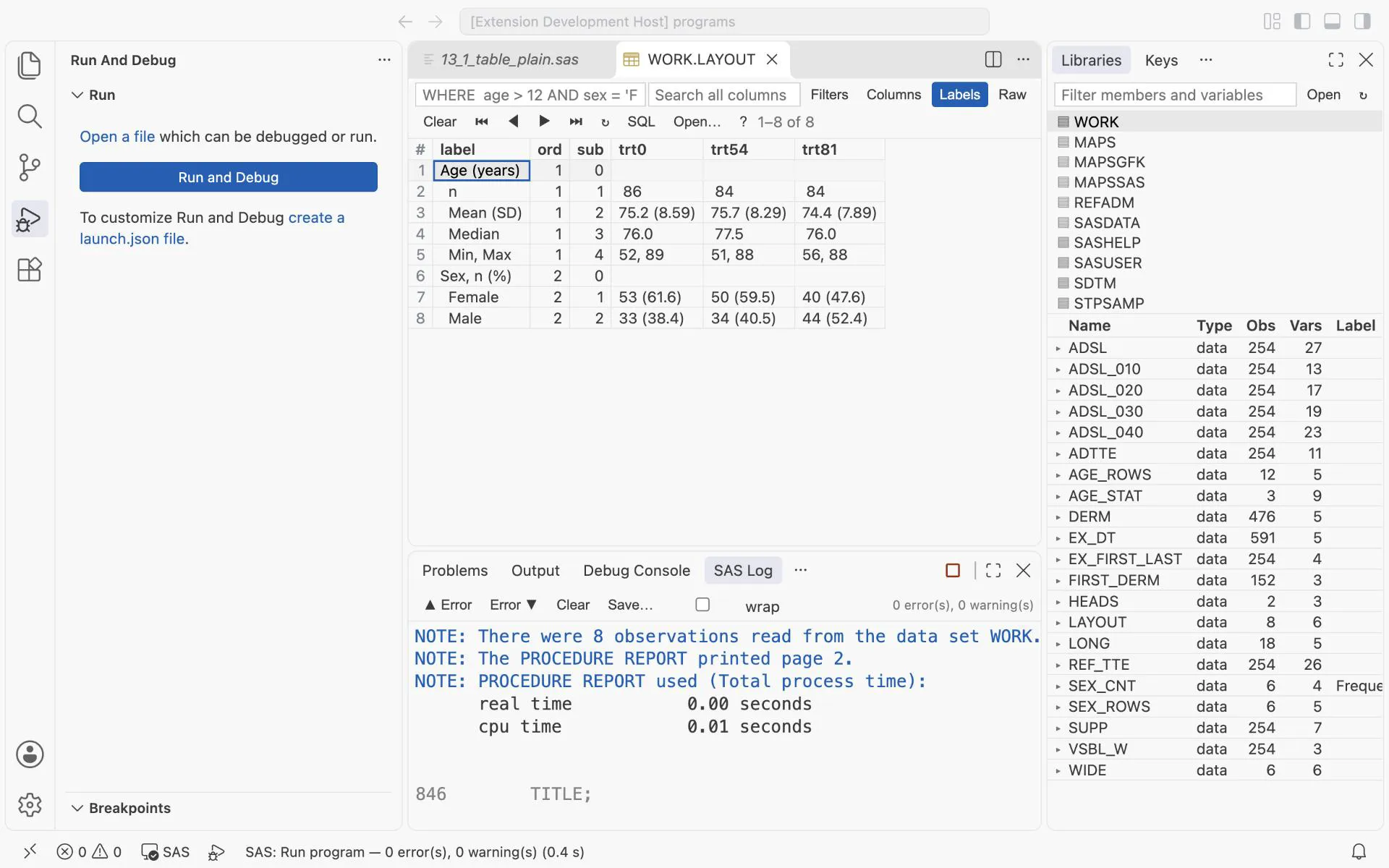
F12 after 13_1_table_plain.sas: WORK.LAYOUT in the data viewer, 8 rows. Each row is one line of the final table: n 86/84/84, Mean (SD) 75.2 (8.59), Female 53 (61.6).

Exercise 13-1. Add race to the table: a categorical section like sex. Print the output of PROC FREQ first. How many rows does it have for the placebo column, and what does the table show for American Indian on placebo?

Exercise 13-2. Add a column “Total” for all subjects. Which of the four jobs change?

13.3 Count subjects, not records: the adverse event table

ADAE has one record per adverse event, and a subject can have many. The table counts subjects: “how many subjects had at least one headache”. COUNT(DISTINCT usubjid) does that (chapter 6).

/* Chapter 13: treatment emergent adverse events by system organ class and preferred term, by hand */

/* Step 010: the big N of each column, from ADSL, into a data set and into macro variables n0 n54 n81 */
PROC SQL;
  CREATE TABLE ae_bign AS
    SELECT trt01an AS trtan, COUNT(DISTINCT usubjid) AS bign
      FROM refadm.adsl
      WHERE saffl = "Y"
      GROUP BY trt01an;
QUIT;
DATA _NULL_;
  SET ae_bign;
  CALL SYMPUTX(CATS("n", trtan), bign);
RUN;

/* Step 020: the treatment emergent events of the safety population */
DATA teae;
  SET refadm.adae(WHERE=(saffl = "Y" AND trtemfl = "Y"));
  KEEP usubjid trtan aebodsys aedecod;
RUN;

/* Step 030: count subjects, not records: overall, per SOC, per SOC and PT */
PROC SQL;
  CREATE TABLE ae_any AS
    SELECT trtan, COUNT(DISTINCT usubjid) AS n
      FROM teae GROUP BY trtan;
  CREATE TABLE ae_soc AS
    SELECT trtan, aebodsys, COUNT(DISTINCT usubjid) AS n
      FROM teae GROUP BY trtan, aebodsys;
  CREATE TABLE ae_pt AS
    SELECT trtan, aebodsys, aedecod, COUNT(DISTINCT usubjid) AS n
      FROM teae GROUP BY trtan, aebodsys, aedecod;
QUIT;

DATA ae_cnt;
  LENGTH aebodsys aedecod $200;
  SET ae_any(IN=in0) ae_soc(IN=in1) ae_pt(IN=in2);
  IF      in0 THEN level = 0;
  ELSE IF in1 THEN level = 1;
  ELSE             level = 2;
RUN;

/* Step 040: every line of the table in every column, with 0 where nobody had the event */
PROC SQL;
  CREATE TABLE ae_grid AS
    SELECT r.level, r.aebodsys, r.aedecod, b.trtan, b.bign, COALESCE(c.n, 0) AS n
      FROM (SELECT DISTINCT level, aebodsys, aedecod FROM ae_cnt) AS r
           CROSS JOIN ae_bign AS b
           LEFT JOIN ae_cnt AS c
             ON  c.level = r.level AND c.aebodsys = r.aebodsys
             AND c.aedecod = r.aedecod AND c.trtan = b.trtan
      ORDER BY r.aebodsys, r.level, r.aedecod, b.trtan;
QUIT;

/* Step 050: the text of each cell and of each row label */
DATA ae_text;
  LENGTH label $200 value $20;
  SET ae_grid;
  IF      level = 0 THEN label = "Subjects with at least one TEAE";
  ELSE IF level = 1 THEN label = aebodsys;
  ELSE                   label = CAT("  ", STRIP(aedecod));  /* STRIP: CAT keeps trailing blanks */
  IF n = 0 THEN value = "0";
  ELSE value = CATX(" ", PUT(n, 4.), CATS("(", PUT(n / bign * 100, 5.1), ")"));
RUN;

/* Step 060: one column per treatment */
PROC TRANSPOSE DATA=ae_text OUT=ae_layout(DROP=_name_) PREFIX=c;
  BY aebodsys level aedecod label;
  ID trtan;
  VAR value;
RUN;

/* Step 070: print */
OPTIONS LS=132 PS=60 NOCENTER;
TITLE1 "Table 14.3.1 Treatment emergent adverse events by system organ class and preferred term";
TITLE2 "Safety population. Subjects are counted once per line.";
/* MISSING: the overall line and the SOC lines have an empty aedecod; without it PROC REPORT drops them */
PROC REPORT DATA=ae_layout NOWD HEADLINE SPLIT="|" MISSING;
  COLUMN aebodsys level aedecod label c0 c54 c81;
  DEFINE aebodsys / ORDER NOPRINT;
  DEFINE level    / ORDER NOPRINT;
  DEFINE aedecod  / ORDER NOPRINT;
  DEFINE label    / DISPLAY "System organ class|  Preferred term" WIDTH=50 FLOW;
  DEFINE c0       / DISPLAY "Placebo|(N=&n0.)"                   WIDTH=20 CENTER;
  DEFINE c54      / DISPLAY "Xanomeline Low Dose|(N=&n54.)"      WIDTH=20 CENTER;
  DEFINE c81      / DISPLAY "Xanomeline High Dose|(N=&n81.)"     WIDTH=20 CENTER;
  COMPUTE AFTER aebodsys;
    LINE " ";
  ENDCOMP;
RUN;
TITLE;

What you should see: a table of six pages. It starts like this:

Table 14.3.1 Treatment emergent adverse events by system organ class and preferred term
Safety population. Subjects are counted once per line.

  System organ class                                        Placebo         Xanomeline Low Dose   Xanomeline High Dose
   Preferred term                                            (N=86)                (N=84)                (N=84)
  --------------------------------------------------------------------------------------------------------------------
  Subjects with at least one TEAE                          65 (75.6)             77 (91.7)             76 (90.5)

  CARDIAC DISORDERS                                        12 (14.0)             13 (15.5)             15 (17.9)
    ATRIAL FIBRILLATION                                     1 (1.2)               1 (1.2)               3 (3.6)
    ATRIAL FLUTTER                                             0                  1 (1.2)               1 (1.2)
    ATRIAL HYPERTROPHY                                      1 (1.2)                  0                     0

The first line is a number you know. 65, 77 and 76 subjects have at least one treatment emergent adverse event (TEAE), as in chapter 6. Five details make this program correct:

Three levels, three counts. One count per treatment, one per system organ class (SOC), one per SOC and preferred term (PT). A subject with two headaches counts once in the PT line. A subject with a headache and a dizziness counts once in the SOC line. Never add the PT lines to get the SOC line.
Step 040 builds a grid. A count exists only where somebody had the event. Nobody on placebo had atrial flutter, so there is no record for it. The CROSS JOIN makes every line in every column, the LEFT JOIN adds the count, and COALESCE(c.n, 0) writes 0 where there is none. Without the grid, that cell would be blank, and a blank is not a 0.
CAT keeps trailing blanks. In this program aedecod is 200 characters long. Step 030 gives it that length with LENGTH aebodsys aedecod $200. In the reference ADAE it has 46. CAT(" ", aedecod) adds two blanks: 2 + 200 = 202 characters. That is too long for the result, so SAS writes a WARNING. STRIP removes the trailing blanks first.
MISSING in PROC REPORT. The first line and the SOC lines have an empty aedecod. PROC REPORT drops every record with a missing value in an ORDER variable. It writes no message. Remove MISSING and run the program again: the table starts with ATRIAL FIBRILLATION.
The order here is alphabetical: SOC, then PT. Many shells ask for the most frequent first (Exercise 13-4).

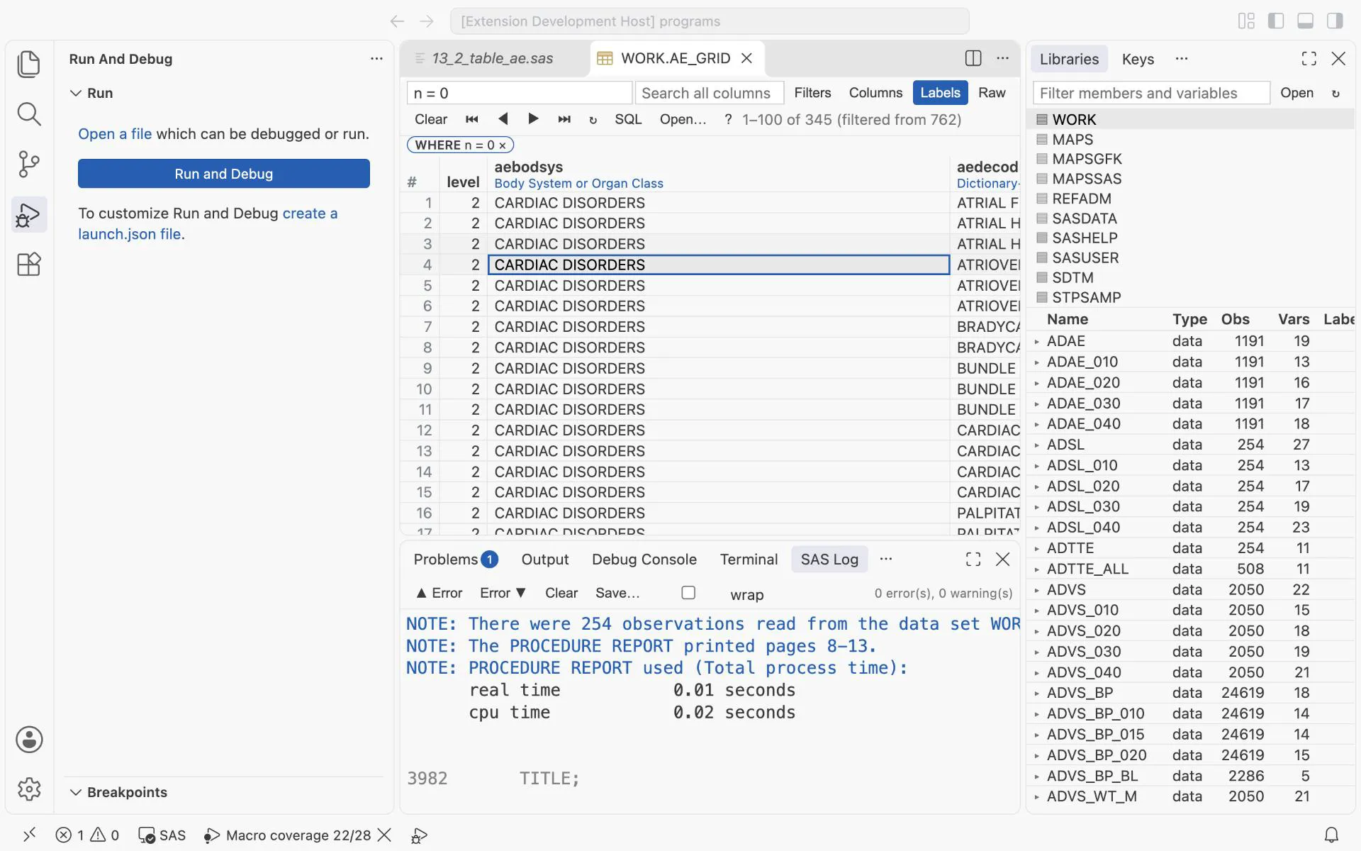
WORK.AE_GRID with WHERE n = 0: 345 of 762 cells exist only because the grid made them. Without the grid they would be missing in the table, not 0.

Exercise 13-3. How many subjects had at least one serious TEAE (aeser = "Y") in each treatment? Count it with PROC SQL. What does the result show for placebo, and why?

Exercise 13-4. Sort the system organ classes by the number of subjects in all three treatments together, the most frequent first. Which three come first?

13.4 The same code three times: write a study macro

Look at the two programs again. Each table repeats the same steps: count, make text, give it an ord and a sub, transpose, print. A study with 50 tables repeats them 50 times, with 50 chances for a different rounding rule. That is the moment to write a macro: when the same code comes back, not before.

The four macros below are small on purpose. The trick is the row layout: every macro writes the same five variables, so the output of any macro can go into the print macro.

Variable	Holds
`col`	the value of the column variable, for example 0, 54 or 81
`ord`	the section of the table: 1 for age, 2 for age group, …
`sub`	the line in the section: 0 for the heading, then 1, 2, …
`label`	the text in the first column
`value`	the text in the cell, for example `65 (75.6)`

Unix tools pass lines of text from one tool to the next; these macros pass rows of this layout. One more rule: every macro that makes rows (%m_bign, %m_desc, %m_freq) has the same parameter names. data= is the input, out= the output, by= the column variable, where= the records. %m_report prints and %m_need checks; they make no rows, so their parameters follow their job.

/* Chapter 13: study macros for summary tables. Run this file once, then 13_4 and 13_5 use the macros. */
/* All macros share one interface: data= the input, out= the output, by= the column variable,       */
/* where= the records to use. Every macro writes rows in one layout, the same for all of them:       */
/*   col (the value of by=), ord (the section), sub (the line in the section), label, value (text)   */

/*******************************************************************************
  Macro       : %m_need
  Purpose     : Check that the required parameters of a macro are not empty.
                Returns 1 (and writes an ERROR line for each empty one) or 0.
  Parameters  :
    macro=      the name of the calling macro, for the message
    params=     the names of the required parameters, separated by blanks
  Example     :
    %IF %m_need(macro=M_FREQ, params=data var by denom) %THEN %RETURN;
  Note        : the local names start with _mn_, so they never hide a
                parameter of the macro that calls %m_need.
*******************************************************************************/
%MACRO m_need(macro=, params=);
  %LOCAL _mn_i _mn_p _mn_bad;
  %LET _mn_bad = 0;
  %DO _mn_i = 1 %TO %SYSFUNC(COUNTW(&params., %STR( )));
    %LET _mn_p = %SCAN(&params., &_mn_i., %STR( ));
    %IF %SUPERQ(&_mn_p.) = %THEN %DO;
      %PUT %STR(ERR)OR: [&macro.] The parameter %UPCASE(&_mn_p.)= is required.;
      %LET _mn_bad = 1;
    %END;
  %END;
  &_mn_bad.
%MEND m_need;

/*******************************************************************************
  Macro       : %m_bign
  Purpose     : The big N: the number of subjects in each column.
  Parameters  :
    data=       the subject level data set, for example refadm.adsl
    by=         the numeric column variable, for example trt01an
    where=      the population, for example saffl = "Y" (default: all records)
    id=         the subject variable (default: usubjid)
    out=        the output data set: one record per column, variables col and bign
*******************************************************************************/
%MACRO m_bign(data=, by=, where=1, id=usubjid, out=);
  %IF %m_need(macro=M_BIGN, params=data by id out) %THEN %RETURN;
  %IF NOT %SYSFUNC(EXIST(&data.)) %THEN %DO;
    %PUT %STR(ERR)OR: [M_BIGN] The data set &data. does not exist.;
    %RETURN;
  %END;

  PROC SQL;
    CREATE TABLE &out. AS
      SELECT &by. AS col, COUNT(DISTINCT &id.) AS bign
        FROM &data.(WHERE=(&where.))
        GROUP BY &by.
        ORDER BY col;
  QUIT;

  DATA _NULL_;
    SET &out.;
    PUTLOG "NOTE: [M_BIGN] column " col "has N=" bign;
  RUN;
%MEND m_bign;

/*******************************************************************************
  Macro       : %m_desc
  Purpose     : Rows for a continuous variable: n, Mean (SD), Median, Min, Max.
  Parameters  :
    data=       the input data set
    var=        the numeric variable
    by=         the numeric column variable
    where=      the records to use (default: all records)
    dec=        the decimals of the collected value (default 0): the mean and
                the median get one more, the SD two more
    label=      the text of the section heading
    ord=        the number of the section in the table
    out=        the output data set in the row layout
*******************************************************************************/
%MACRO m_desc(data=, var=, by=, where=1, dec=0, label=, ord=, out=);
  %IF %m_need(macro=M_DESC, params=data var by dec label ord out) %THEN %RETURN;
  %IF NOT %SYSFUNC(EXIST(&data.)) %THEN %DO;
    %PUT %STR(ERR)OR: [M_DESC] The data set &data. does not exist.;
    %RETURN;
  %END;

  /* Step 010: the statistics, one record per column */
  PROC MEANS DATA=&data.(WHERE=(&where.)) NOPRINT NWAY;
    CLASS &by.;
    VAR &var.;
    OUTPUT OUT=_md_010 N=n MEAN=mean STD=sd MEDIAN=median MIN=min MAX=max;
  RUN;

  /* Step 020: five lines of text per column */
  DATA &out.;
    LENGTH label $60 value $20;
    SET _md_010(RENAME=(&by.=col));
    ord = &ord.;
    sub = 0; label = "&label.";    value = " ";                                    OUTPUT;
    sub = 1; label = "  n";         value = CATS(n);                                OUTPUT;
    sub = 2; label = "  Mean (SD)"; value = CATX(" ", PUT(mean, 8.%EVAL(&dec. + 1)),
                                              CATS("(", PUT(sd, 8.%EVAL(&dec. + 2)), ")")); OUTPUT;
    sub = 3; label = "  Median";    value = STRIP(PUT(median, 8.%EVAL(&dec. + 1))); OUTPUT;
    sub = 4; label = "  Min, Max";  value = CATX(", ", PUT(min, 8.&dec.), PUT(max, 8.&dec.)); OUTPUT;
    KEEP col ord sub label value;
  RUN;

  PROC DATASETS LIBRARY=work NOLIST NOWARN; DELETE _md_:; RUN; QUIT;
%MEND m_desc;

/*******************************************************************************
  Macro       : %m_freq
  Purpose     : Rows for a categorical variable: n (%) of the big N, with a
                line for every category in every column, also when n is 0.
  Parameters  :
    data=       the input data set
    var=        the categorical variable
    by=         the numeric column variable
    where=      the records to use (default: all records)
    id=         count distinct values of this variable (for example usubjid);
                empty (default): count records
    denom=      the big N data set from %m_bign (variables col and bign)
    fmt=        a format for the category text (default: the value itself)
    orderby=    the variable that gives the order of the categories
                (default: var=), for example agegr1n for agegr1
    label=      the text of the section heading (", n (%)" is added)
    ord=        the number of the section in the table
    out=        the output data set in the row layout
*******************************************************************************/
%MACRO m_freq(data=, var=, by=, where=1, id=, denom=, fmt=, orderby=, label=, ord=, out=);
  %LOCAL count;
  %IF %m_need(macro=M_FREQ, params=data var by denom label ord out) %THEN %RETURN;
  %IF NOT %SYSFUNC(EXIST(&data.)) %THEN %DO;
    %PUT %STR(ERR)OR: [M_FREQ] The data set &data. does not exist.;
    %RETURN;
  %END;
  %IF %SUPERQ(orderby) = %THEN %LET orderby = &var.;
  /* count subjects (id=) or records: the SQL text is chosen before the step */
  %IF %SUPERQ(id) NE %THEN %LET count = COUNT(DISTINCT &id.);
  %ELSE                    %LET count = COUNT(*);

  PROC SQL;
    /* Step 010: the counts that exist in the data */
    CREATE TABLE _mf_010 AS
      SELECT &by. AS col, &var. AS level, &orderby. AS lorder,
             &count. AS n
        FROM &data.(WHERE=(&where.))
        WHERE NOT MISSING(&var.)
        GROUP BY 1, 2, 3;
    /* Step 020: every category in every column */
    CREATE TABLE _mf_020 AS
      SELECT d.col, d.bign, l.level, l.lorder
        FROM &denom. AS d, (SELECT DISTINCT level, lorder FROM _mf_010) AS l;
    /* Step 030: the count, 0 where the data has none */
    CREATE TABLE _mf_030 AS
      SELECT a.*, COALESCE(c.n, 0) AS n
        FROM _mf_020 AS a LEFT JOIN _mf_010 AS c
          ON a.col = c.col AND a.level = c.level
        ORDER BY a.col, a.lorder, a.level;
  QUIT;

  /* Step 040: one heading line and one line per category, in every column */
  DATA &out.;
    LENGTH label $60 value $20;
    SET _mf_030;
    BY col;
    ord = &ord.;
    IF FIRST.col THEN DO;
      sub = 0; label = "&label., n (%)"; value = " "; OUTPUT;
    END;
    sub + 1;
    label = CAT("  ", %IF %SUPERQ(fmt) NE %THEN STRIP(PUT(level, &fmt.)); %ELSE CATS(level););
    IF n = 0 THEN value = "0";
    ELSE value = CATX(" ", PUT(n, 4.), CATS("(", PUT(n / bign * 100, 5.1), ")"));
    OUTPUT;
    KEEP col ord sub label value;
  RUN;

  PROC DATASETS LIBRARY=work NOLIST NOWARN; DELETE _mf_:; RUN; QUIT;
%MEND m_freq;

/*******************************************************************************
  Macro       : %m_report
  Purpose     : Print rows in the row layout as a table: one line per ord and
                sub, one column per value of col, headers with the big N.
  Parameters  :
    data=       the rows (variables col, ord, sub, label, value)
    denom=      the big N data set from %m_bign (variables col and bign)
    fmt=        the format that turns col into the column name
    lwidth=     the width of the label column (default 32)
    cwidth=     the width of each treatment column (default 20)
*******************************************************************************/
%MACRO m_report(data=, denom=, fmt=, lwidth=32, cwidth=20);
  %LOCAL i _mr_n;
  %IF %m_need(macro=M_REPORT, params=data denom fmt lwidth cwidth) %THEN %RETURN;

  /* Step 010: one column per value of col */
  PROC SORT DATA=&data. OUT=_mr_010; BY ord sub label; RUN;
  PROC TRANSPOSE DATA=_mr_010 OUT=_mr_020(DROP=_name_) PREFIX=c;
    BY ord sub label;
    ID col;
    VAR value;
  RUN;

  /* Step 020: the column names and headers, from the big N */
  DATA _NULL_;
    SET &denom. END=eof;
    CALL SYMPUTX(CATS("_mr_c", _N_), col, "L");
    CALL SYMPUTX(CATS("_mr_h", _N_), CATS(PUT(col, &fmt.), "|(N=", bign, ")"), "L");
    IF eof THEN CALL SYMPUTX("_mr_n", _N_, "L");
  RUN;

  /* Step 030: print */
  PROC REPORT DATA=_mr_020 NOWD HEADLINE SPLIT="|" MISSING;
    COLUMN ord sub label %DO i = 1 %TO &_mr_n.; c&&_mr_c&i. %END;;
    DEFINE ord   / ORDER NOPRINT;
    DEFINE sub   / ORDER NOPRINT;
    DEFINE label / DISPLAY " " WIDTH=&lwidth. FLOW;
    %DO i = 1 %TO &_mr_n.;
      DEFINE c&&_mr_c&i. / DISPLAY "&&_mr_h&i." WIDTH=&cwidth. CENTER;
    %END;
    COMPUTE AFTER ord;
      LINE " ";
    ENDCOMP;
  RUN;

  PROC DATASETS LIBRARY=work NOLIST NOWARN; DELETE _mr_:; RUN; QUIT;
%MEND m_report;

Run this file once with F4. It only defines the macros: the log shows no step. Five things to notice:

%m_need checks the required parameters of the other four. It is a function-style macro: it runs no step and returns a value, 1 or 0, where it is called: %IF %m_need(...) %THEN %RETURN;. Its local names start with _mn_, so they cannot hide the caller’s parameters. A macro that reads its caller’s parameters must never use the same names (see the list processing case study). %m_need exists because the loop that checks required parameters was already copied three times in Part II, into %m_iso_dt, %m_chg and %m_tte. The third copy is the moment to write the tool.
%m_bign writes the big N to the log, so every table program shows its population: NOTE: [M_BIGN] column 0 has N=86.
%m_desc follows the decimal rule of 13.2 with one parameter: dec= is the decimals of the collected value.
%m_freq builds the grid of 13.3, so every category has a line in every column, with 0 where nobody is. orderby= gives the order of the categories, and id=usubjid makes it count subjects instead of records.
%m_report prints any rows in the layout, and takes the column headers from the big N data set.

Each macro also cleans up. Its work data sets start with its own prefix: _md_, _mf_ or _mr_. At the end, it deletes them with DELETE _md_:;.

Exercise 13-5. Call %m_freq without denom=. What does the log say, and does the output data set exist?

Exercise 13-6. A new shell asks for percents with no decimals. In 13.2 you would change every table program. Where do you change it now?

13.5 The demographics table again

/* Chapter 13: the demographics table again, with the study macros of 13_3_table_macros.sas */

PROC FORMAT;
  VALUE trtf  0 = "Placebo" 54 = "Xanomeline Low Dose" 81 = "Xanomeline High Dose";
  VALUE $sexf "F" = "Female" "M" = "Male";
RUN;

/* Compute and arrange: one macro call per section of the table */
%m_bign(data=refadm.adsl, by=trt01an, where=saffl = "Y", out=dm_bign)

%m_desc(data=refadm.adsl, var=age, by=trt01an, where=saffl = "Y",
        label=Age (years), ord=1, out=dm_age)
%m_freq(data=refadm.adsl, var=agegr1, orderby=agegr1n, by=trt01an, where=saffl = "Y",
        denom=dm_bign, label=Age group, ord=2, out=dm_agegr1)
%m_freq(data=refadm.adsl, var=sex, by=trt01an, where=saffl = "Y",
        denom=dm_bign, fmt=$sexf., label=Sex, ord=3, out=dm_sex)
%m_freq(data=refadm.adsl, var=race, orderby=racen, by=trt01an, where=saffl = "Y",
        denom=dm_bign, label=Race, ord=4, out=dm_race)

DATA dm_rows;
  SET dm_age dm_agegr1 dm_sex dm_race;
RUN;

/* Print */
OPTIONS LS=110 PS=60 NOCENTER;
TITLE1 "Table 14.1.1 Demographics (safety population)";
%m_report(data=dm_rows, denom=dm_bign, fmt=trtf., lwidth=40)
TITLE;

What you should see:

Table 14.1.1 Demographics (safety population)

                                                  Placebo         Xanomeline Low Dose   Xanomeline High Dose
                                                   (N=86)                (N=84)                (N=84)
  ----------------------------------------------------------------------------------------------------------
  Age (years)
    n                                                86                    84                    84
    Mean (SD)                                   75.2 (8.59)           75.7 (8.29)           74.4 (7.89)
    Median                                          76.0                  77.5                  76.0
    Min, Max                                       52, 89                51, 88                56, 88

  Age group, n (%)
    <65                                          14 (16.3)              8 (9.5)              11 (13.1)
    65-80                                        42 (48.8)             47 (56.0)             55 (65.5)
    >80                                          30 (34.9)             29 (34.5)             18 (21.4)

  Sex, n (%)
    Female                                       53 (61.6)             50 (59.5)             40 (47.6)
    Male                                         33 (38.4)             34 (40.5)             44 (52.4)

  Race, n (%)
    WHITE                                        78 (90.7)             78 (92.9)             74 (88.1)
    BLACK OR AFRICAN AMERICAN                     8 (9.3)               6 (7.1)               9 (10.7)
    AMERICAN INDIAN OR ALASKA NATIVE                 0                     0                  1 (1.2)

Prove it before you trust it. Age and sex are the same as in 13.2, number for number: two programs, written two ways, agree. That is the habit of chapter 15 in small. You can do two more checks by eye. Each section adds up to the big N: 78 + 8 + 0 = 86 for race on placebo. And the American Indian row shows 0, not a blank.

Two details:

orderby=agegr1n. agegr1 is text, and text sorts 65-80 before <65. ADSL keeps a numeric twin, agegr1n, for exactly this.
lwidth=40. With the default width of 32, AMERICAN INDIAN OR ALASKA NATIVE wraps over two lines.

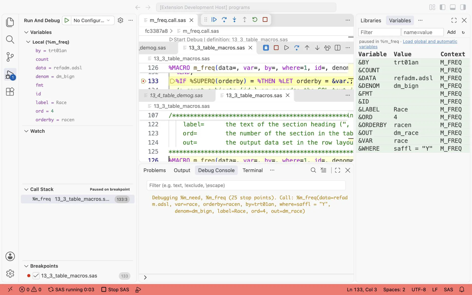
The macro debugger in %m_freq for the race section, called from 13_4_table_demog.sas and stopped at %IF %SUPERQ(orderby): var = race, orderby = racen, denom = dm_bign, label = Race.

13.6 The payoff: a second table

By hand, the demographics table took 81 lines for two sections: age and sex. With the macros it took 28 lines for four sections: age, age group, sex and race. The 28 lines do not count the macros themselves: 13_3_table_macros.sas has 224 lines, but you write it once and every table uses it. A new table is a list of calls: the program below has 43 lines, most of them calls. This one mixes ADSL (one record per subject) and ADVS (one record per subject, parameter, visit and position): the where= picks the baseline.

/* Chapter 13: a second table with the same macros: baseline characteristics from ADSL and ADVS */

PROC FORMAT;
  VALUE trtf 0 = "Placebo" 54 = "Xanomeline Low Dose" 81 = "Xanomeline High Dose";
RUN;

%m_bign(data=refadm.adsl, by=trt01an, where=saffl = "Y", out=bl_bign)

/* BMIBLGR1 is text, and text sorts "25-<30" before "<25". ADSL has no numeric twin: make one */
DATA bl_adsl;
  SET refadm.adsl(WHERE=(saffl = "Y"));
  bmiblgr1n = WHICHC(bmiblgr1, "<25", "25-<30", ">=30");
RUN;

/* From ADSL: one record per subject */
%m_desc(data=refadm.adsl, var=heightbl, by=trt01an, where=saffl = "Y", dec=1,
        label=Height (cm), ord=1, out=bl_height)
%m_desc(data=refadm.adsl, var=weightbl, by=trt01an, where=saffl = "Y", dec=1,
        label=Weight (kg), ord=2, out=bl_weight)
%m_desc(data=refadm.adsl, var=bmibl, by=trt01an, where=saffl = "Y", dec=1,
        label=BMI (kg/m2), ord=3, out=bl_bmi)
%m_freq(data=bl_adsl, var=bmiblgr1, orderby=bmiblgr1n, by=trt01an,
        denom=bl_bign, label=BMI group, ord=4, out=bl_bmigr)

/* From ADVS: one record per subject, parameter, visit and position: the WHERE picks the baseline */
%m_desc(data=refadm.advs, var=aval, by=trtan,
        where=saffl = "Y" AND ablfl = "Y" AND paramcd = "SYSBP" AND atptn = 815,
        label=Systolic BP lying (mmHg), ord=5, out=bl_sysbp)
%m_desc(data=refadm.advs, var=aval, by=trtan,
        where=saffl = "Y" AND ablfl = "Y" AND paramcd = "DIABP" AND atptn = 815,
        label=Diastolic BP lying (mmHg), ord=6, out=bl_diabp)
%m_desc(data=refadm.advs, var=aval, by=trtan,
        where=saffl = "Y" AND ablfl = "Y" AND paramcd = "PULSE" AND atptn = 815,
        label=Pulse lying (beats/min), ord=7, out=bl_pulse)

DATA bl_rows;
  SET bl_height bl_weight bl_bmi bl_bmigr bl_sysbp bl_diabp bl_pulse;
RUN;

OPTIONS LS=110 PS=60 NOCENTER;
TITLE1 "Table 14.1.3 Baseline characteristics (safety population)";
%m_report(data=bl_rows, denom=bl_bign, fmt=trtf.)
TITLE;

What you should see (the first sections, then the blood pressure):

Table 14.1.3 Baseline characteristics (safety population)

                                          Placebo         Xanomeline Low Dose   Xanomeline High Dose
                                           (N=86)                (N=84)                (N=84)
  --------------------------------------------------------------------------------------------------
  Height (cm)
    n                                        86                    84                    84
    Mean (SD)                         162.57 (11.522)       163.43 (10.419)       165.82 (10.131)
    Median                                 162.60                162.60                165.10
    Min, Max                            137.2, 185.4          135.9, 195.6          146.1, 190.5

  Weight (kg)
    n                                        86                    83                    84
    Mean (SD)                          62.76 (12.772)        67.28 (14.124)        70.00 (14.653)
    Median                                 60.55                 64.90                 69.20
    Min, Max                             34.0, 86.2           45.4, 106.1           41.7, 108.0

  BMI (kg/m2)
    n                                        86                    83                    84
    Mean (SD)                          23.64 (3.672)         25.06 (4.271)         25.35 (4.158)
    Median                                 23.40                 24.30                 24.80
    Min, Max                             15.1, 33.3            17.7, 40.1            13.7, 34.5

  BMI group, n (%)
    <25                                  59 (68.6)             47 (56.0)             44 (52.4)
    25-<30                               21 (24.4)             27 (32.1)             28 (33.3)
    >=30                                  6 (7.0)              10 (11.9)             12 (14.3)

  Systolic BP lying (mmHg)
    n                                        85                    84                    84
    Mean (SD)                          138.6 (16.75)         138.8 (16.55)         140.1 (17.82)
    Median                                 140.0                 138.0                 141.0
    Min, Max                              90, 180               100, 178              100, 188

Three things this table teaches:

n is not N. Weight has n = 83 on the low dose, out of N = 84: subject 01-702-1082 has no baseline weight in ADSL. Systolic blood pressure has n = 85 on placebo: subject 01-718-1150 had no BASELINE visit. They are the two subjects for whom %m_baseline of chapter 10 finds a baseline at screening. The table shows n and N, so a reader sees the gap. One trap remains: the BMI group counts 84 on the low dose, not 83. The reference ADSL puts 01-702-1082, who has no BMI, into <25: a missing value is smaller than every number (2.4).
Text sorts as text. bmiblgr1 sorts 25-<30, <25, >=30, and ADSL has no numeric twin. The DATA step bl_adsl makes one: WHICHC returns the position of the value in a list, 1, 2 or 3.
The same macro, two data sets. %m_desc reads ADSL with by=trt01an and ADVS with by=trtan. In the rows both become col, so they print in the same columns.

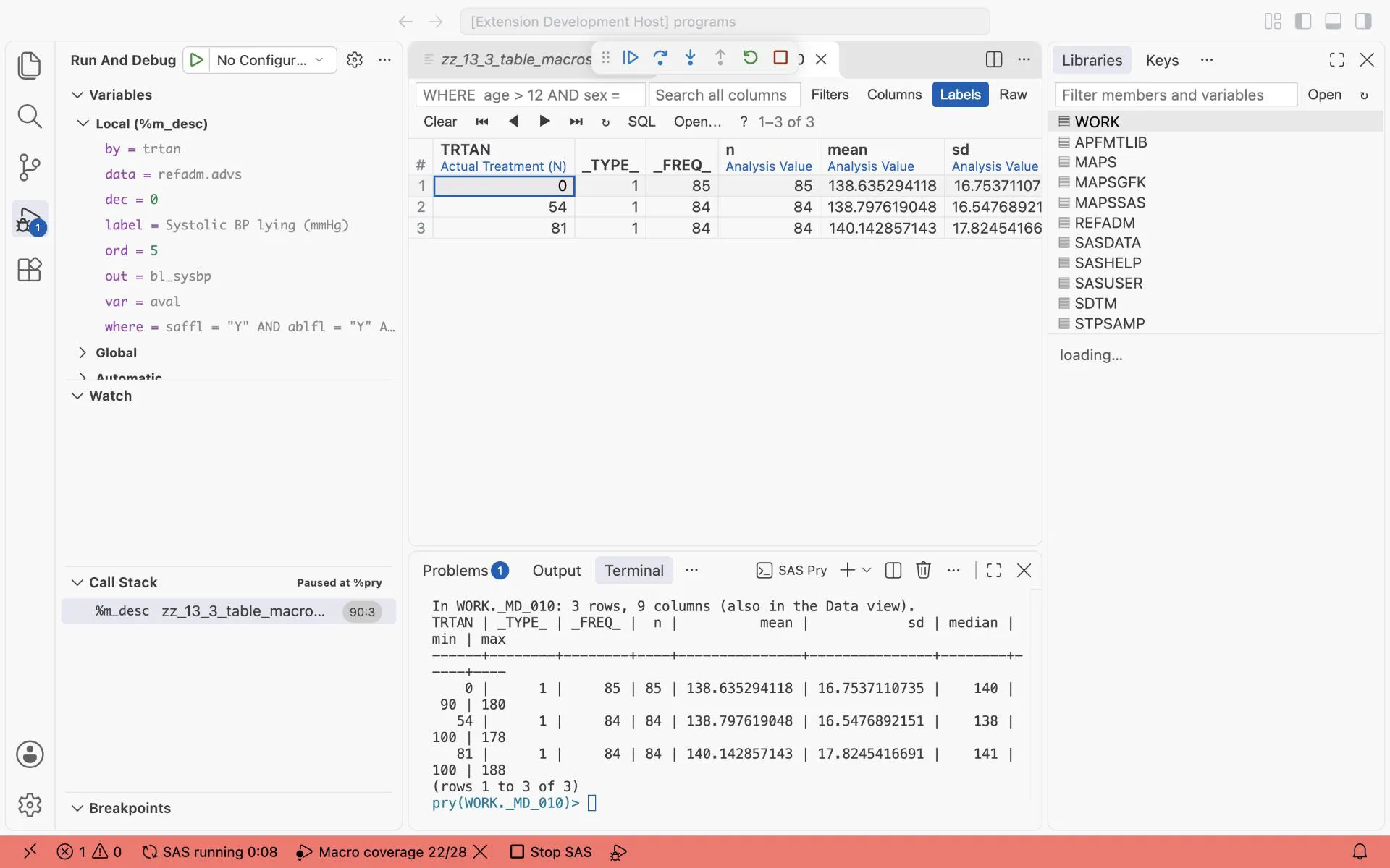
%pry in %m_desc for the section ord = 5: vt _md_010 shows n = 85, 84 and 84 for systolic blood pressure lying, one record per treatment column.

Exercise 13-7. Add the years of education (educlvl in ADSL) to the table as section 8. How many lines of code do you add?

13.7 P-values in a table

Many tables end with a p-value: the TEAE table with a test across the treatments, an efficacy table with the result of a model. The statistician chooses the test and writes it in the SAP. The programmer runs it, takes the number from SAS, and puts it in the table. You do not need the statistics theory for that. You need to know where the number comes from and what to check.

Two terms come up below. An ANCOVA (analysis of covariance) is a linear model: here it explains the change from baseline by the treatment, with the baseline value as a covariate. Least squares means (LS means) are the treatment means from that model, adjusted to the same baseline for every arm. SAS prints them with LSMEANS in PROC GLM.

/* Chapter 13: p-values for a table, Fisher's exact test and an ANCOVA, captured with ODS OUTPUT */

/* Step 010: one record per subject of the safety population, any TEAE yes (1) or no (0) */
PROC SORT DATA=refadm.adae(WHERE=(saffl = "Y" AND trtemfl = "Y")) OUT=st_ae(KEEP=usubjid) NODUPKEY;
  BY usubjid;
RUN;
DATA st_subj;
  MERGE refadm.adsl(IN=insl WHERE=(saffl = "Y") KEEP=usubjid saffl trt01an)
        st_ae(IN=inae);
  BY usubjid;
  IF insl;
  IF inae THEN anyteae = 1;
  ELSE         anyteae = 0;
RUN;

/* Step 020: Fisher's exact test, treatment by any TEAE. ODS OUTPUT keeps the result as a data set */
ODS OUTPUT FishersExact=st_fisher;
PROC FREQ DATA=st_subj;
  TABLES trt01an * anyteae / NOROW NOPERCENT;
  EXACT FISHER;
RUN;
PROC PRINT DATA=st_fisher NOOBS;
RUN;

/* Step 030: ANCOVA, change from baseline in systolic BP (lying) at Week 24, baseline as covariate */
DATA st_bp;
  SET refadm.advs(WHERE=(paramcd = "SYSBP" AND atptn = 815 AND avisit = "Week 24"
                         AND NOT MISSING(chg) AND NOT MISSING(base)));
RUN;
/* PLOTS=NONE: no diagnostic graphs. They need a folder SAS can write to, and the table does not use them */
ODS OUTPUT ModelANOVA=st_anova LSMeans=st_lsm Diff=st_diff;
PROC GLM DATA=st_bp PLOTS=NONE;
  CLASS trtpn;
  MODEL chg = trtpn base / SS3;
  LSMEANS trtpn / PDIFF STDERR;
RUN;
QUIT;
PROC PRINT DATA=st_anova NOOBS;
  WHERE hypothesistype = 3;
  VAR dependent source df ss fvalue probf;
RUN;
PROC PRINT DATA=st_lsm NOOBS;
RUN;
PROC PRINT DATA=st_diff NOOBS;
RUN;

/* Step 040: a p-value row for the table, formatted the way tables show it */
DATA st_prow;
  SET st_fisher(WHERE=(name1 = "XP2_FISH"));
  LENGTH label $60 value $20;
  label = "p-value (Fisher's exact test)";
  value = STRIP(PUT(nvalue1, PVALUE6.4));
  KEEP label value nvalue1;
RUN;
PROC PRINT DATA=st_prow NOOBS;
RUN;

What you should see: the counts of the TEAE table again, as a 3 × 2 table, then the Fisher’s exact test:

Table of TRT01AN by anyteae          anyteae 0    anyteae 1    Total
0  (placebo)                                21           65       86
54 (low dose)                                7           77       84
81 (high dose)                               8           76       84

Fisher's Exact Test
Table Probability (P)       0.0002
Pr <= P                     0.0056

The p-value of the test is Pr <= P: 0.0056. Then the ANCOVA. 115 subjects have a change at Week 24. The treatment effect has p = 0.4846. The least squares means are −1.75 (placebo), −1.40 (low dose) and −5.29 (high dose) mmHg.

Three new things in this program:

ODS OUTPUT keeps a result as a data set. Every table that a procedure prints is an ODS output object. Each has a name, for example FishersExact, ModelANOVA, LSMeans or Diff. ODS OUTPUT FishersExact=st_fisher; before the step writes that table to WORK.ST_FISHER. Then a DATA step takes the number from the data set, never from the printed page. To find the name of a table, run the step once between ODS TRACE ON; and ODS TRACE OFF;: the log lists the name of every table. Chapter 14 uses the same statement for the Kaplan-Meier quartiles.
PVALUE6.4 formats a p-value. It prints 0.0056 as 0.0056 and a very small value as <.0001, the way tables show it. Never round a p-value with ROUND: 0.00004 would become 0.0000.
PLOTS=NONE on PROC GLM. Without it, GLM draws diagnostic graphs and writes them to a folder. On SAS OnDemand that folder is not writable: the log shows ERROR: Cannot write image ..., and GLM stops before the LSMEANS statement. So the LSMeans and Diff data sets are not made, and the log says WARNING: Output 'LSMeans' was not created. The table does not need the graphs: switch them off.

Before you put a p-value in a table, check four things:

The subjects. The log of PROC GLM says Number of Observations Used 115. The table must show the same subjects: here the 115 subjects with a change at Week 24 (58 + 27 + 30 in the subgroup table).
The test and the model. Fisher’s exact test, not chi-square; chg = trtpn base, as the SAP says. A wrong word in the MODEL statement gives a p-value too, and it looks just as real.
The order of the treatments. The Diff data set compares level 1 with level 3 (placebo with high dose: 0.2730). Which comparison the table needs is in the SAP.
The format. PVALUE6.4, from the data set, in the cell the shell shows.

Exercise 13-8. Make the same Fisher’s exact test for subjects with at least one severe TEAE. What is the p-value?

Exercise 13-9. Run the PROC GLM step between ODS TRACE ON; and ODS TRACE OFF;. What is the name of the table with the type III tests, and what is its label?

13.8 Your company’s library

The macros of a company library do the same four jobs, with more options. Examples are a Total column, event counts next to subject counts, sorting by frequency, RTF and PDF output, and the company’s page header. At a new company, open its table macros and find the four jobs. Where is the big N? Where are the statistics? Where is the row layout? Where is the PROC REPORT? And when the SAP asks for something the library cannot do, you can still write the table: you just did.

Exercises

Each exercise is next to the program it changes:

Exercises	Program
13-1, 13-2	`13_1_table_plain.sas`
13-3, 13-4	`13_2_table_ae.sas`
13-5, 13-6	`13_3_table_macros.sas`
13-7	`13_5_table_baseline.sas`
13-8, 13-9	`13_6_table_stats.sas`

The answers are in Answers, Part III.